Two-Dimension Mesh Convergence in Ansys Workbench

One of our experts has volunteered to help you in your engineering classes and has created a small step-by-step guide for you. In the following sample you can learn how to create a simple two-dimensional mesh convergence in Ansys Workbench to stimulate the boundary layer on a flat plate.

We know that creating a two-dimensional mesh convergence in Ansys Workbench can be hard, so if you can’t manage the assignment, there is no reason to panic! With Assignment.EssayShark.com you can get expert assistance with any assignment on any discipline. You can choose the best expert to perform the task and chat with your expert during the writing process. Every order is completed individually for every customer, and we guarantee a high-quality result. If you are seeking expert help, rely on our team of experts and receive a totally unique paper that corresponds with your needs.

Simulating the Boundary Layer on a Flat Plate

Task: Using Ansys Workbench, create a simple two-dimensional mesh that is used to simulate the boundary layer on a flat plate.

Solution:

This guide will show in steps what needs to be done to get to the final result.

Creating a new FLUENT project

1. Launch the program.
2. In Toolbox Customization under Analysis Systems, verify that “Fluid Flow” has a check mark next to it.
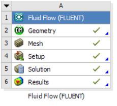
3. In the Toolbox Fluid Flow (FLUENT) hold LMB to drag it into the box that will appear in Project Schematic. If everything works correctly, there will now be a Fluid Flow (FLUENT) template in Project Schematic.
4. In the new window under Advanced Geometry Options, and to the right of option Analysis Type, choose 3D and then 2D from the drop-down menu. This limits the analysis to two dimensions.
5. Double click “Geometry” in the newly created Fluid Flow (FLUENT) template to open ANSYS Design Modeler.

Creating the required edges in Design Modeler

At startup, Design Modeler will prompt the user to select a desired length unit. Click LMB on the circle next to “Meter,” then click OK.

1. In Tree Outline, choose XY Plane. Then in Display Toolbar (near the top), look at Face/Plane/Sketch.
2. Choose Box Zoom from the Display Toolbar. Use LMB to drag a box from the 3rd quadrant, near the origin, to the approximate coordinates (1, 1). The resulting view of the first quadrant will be perfect for constructing the sketch.
3. Choose Sketching, which is located near the bottom of Tree Outline. This will bring up the Draw tab of Sketching Toolboxes.
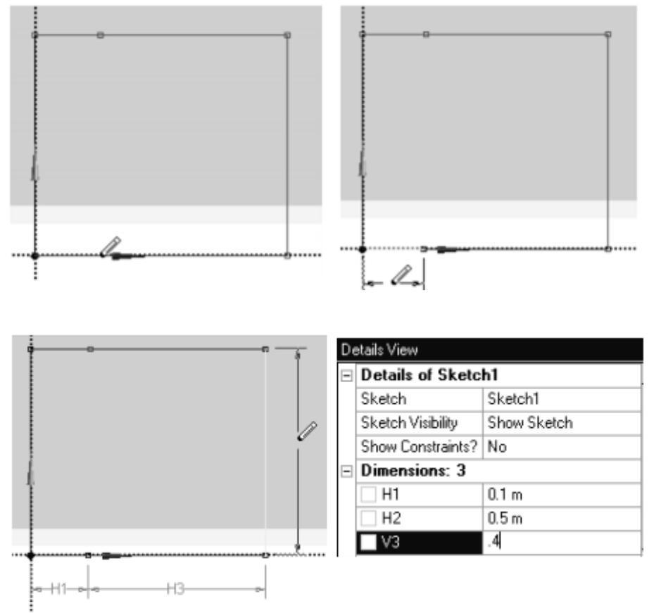
4. Choose Rectangle and hover over the origin. Click LMB when a “P” is displayed. Move the cursor to make a rectangle in the 1st quadrant that is about .5 m by .5 m. Click LMB to place the other corner of the rectangle.

Splitting edges and their dimensions

1. In Sketching Toolboxes, and with Modify-Split, about ¼ of the way from the left edge, click LMB on the top edge and then again in the same location on the bottom edge.
2. In Sketching Toolboxes, Dimensions (when Dimensions opens, the default is “General,” which is what we want), click LMB on the short section of the bottom edge. Then, move the cursor below the bottom edge and click LMB again to place the dimension at the cursor’s location (see figures above).
3. Click LMB on the long section of the bottom edge. Move the cursor below this edge and click LMB again to place the dimension. Repeat this process for the dimension in the right edge of the rectangle.
4. In the Dimensions section of Details View, the first dimension listed corresponds to the length of the symmetry boundary. Set this value to “0.1” m. The second dimension corresponds to the length of the plate; set it to “.5” m. The last dimension corresponds to the rectangle height; set it to “.4” m.
5. In Sketching Toolboxes, with Constraints-Equal Length, click LMB on the short section of the rectangle’s bottom edge, which will serve as the symmetry boundary, and then again on the corresponding short section of the top edge.

Creating of the surface from the sketch

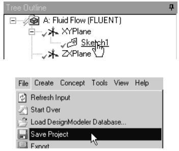
1. In Concept (in DM’s main menu bar), Surfaces from Sketches then Sketch 1 from Tree Outline under XY Plane, Apply in the Details View to set “Sketch 1” as the Base Object.
2. The default settings are acceptable, so choose Generate from the toolbar near the top to create the surface; the surface should turn gray.
3. In the upper left corner of the DM, choose File>Save Project. After selecting an appropriate folder to save the project in, enter “Flat Plate” for the File Name, then Save. Close the DM window.

Setting meshing options and label the edges

1. Open ANSYS Meshing by Mesh in Project Schematic.
2. From the Meshing Options window that opens, click LMB on the circle next to “Tetrahedrons (Patch Independent)” to set the Mesh Method, then OK.
3. From anywhere in the Graphics window, click RMB on View, and then Front. This will orient the geometry so it will be easier to work with.
4. From the Selection Toolbar, which is located near the top of the ANSYS Meshing window, select Edge to change the selection filter from “Face” to “Edge.”
5. Place the cursor over the left edge of the rectangle. When the edge changes to a dotted red line, click LMB to select it. The edge will turn green to indicate that it has been selected. Then click RMB again in the same spot, Create Named Selection, and enter “inlet” as the name for that edge; click OK.
6. Repeat the process in the previous step to name the lower left edge “symmetry,” the lower right edge “plate,” and the right edge “outlet.”
7. Name the two edges that form the top of the rectangle “top left” and “top right.”

Insert a mapped face mesh and sizing controls

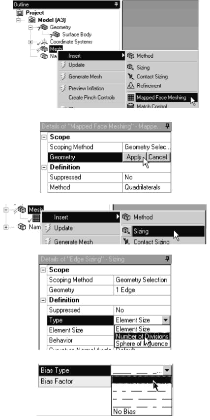
1. From Outline, click RMB on Mesh>Insert>Mapped Face Meshing.
2. Click LMB on the front surface of the geometry. In Details of “Mapped Face Meshing,” apply to make this surface the Geometry selection. Check so that Method is set to “Quadrilaterals.”
3. Click RMB on Mesh>Insert>Sizing. From the Display Toolbar, under Edge, click LMB on the left edge that we had labeled “inlet” and Apply.
4. Change Type from “Element Size” to “Number of Divisions” and then set Number of Divisions to “30.”
5. For Bias Type, it is No Bias, then click LMB on the down arrow to display the available Bias Types. Click LMB on the first option available in the drop down menu. Enter “10” for the value of Bias Factor.
6. Repeat the procedure of the last three steps to put 30 divisions on the right edge that we labeled “outlet” with one exception: for Bias Type, click LMB for the second option available from the drop down menu instead of the first, or else the bias will be in the wrong direction.
7. Put 10 divisions on the bottom left edge that we labeled “symmetry.” Choose the first Bias Type from the drop-down menu so that a finer mesh is produced near the leading edge of the plate. Enter a Bias Factor of 15.
8. Repeat the procedure from the previous step for the top left edge that we labeled “top left” but use the second Bias Type on the drop-down menu.
9. Lastly, put 30 divisions on the two remaining edges, “plate” and “top right.” Use a Bias Factor of 15 with the Bias Type; it will give a finer mesh near the leading edge of the plate. At this point there should be a total of six Edge Sizing entries listed in Outline.
10. Click RMB on Mesh>Generate Mesh. This generates a mesh made up of rectangular elements that get progressively finer (the mesh is clustered) near the leading edge of the plate.
11. In the upper left corner of the Meshing window, go to File>Save Project, then close ANSYS Meshing.

Update mesh and launch FLUENT

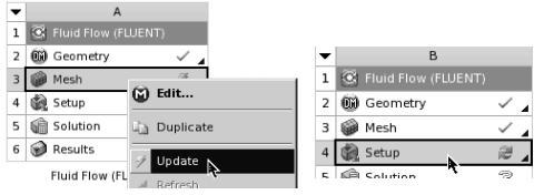
1. In the Project Schematic of ANSYS Workbench, click RMB on Mesh from the analysis template, then Update. A check mark should now appear to the right of both Geometry and Mesh.
2. Choose Setup from the Project Schematic to open FLUENT Launcher. In FLUENT Launcher, verify that the box next to “Double Precision” is selected, then click OK.
3. The next screen will be the main FLUENT Window with your mesh in the Graphics Window.

Define the fluid as liquid water

1. The default fluid is air, but we want to define the fluid as water. In the main FLUENT menu, go through Define>Materials>Create/Edit>FLUENT Database. Select water liquid from the list of FLUENT Database Materials. Copy.
2. Write down the density and viscosity of liquid water. These properties are needed later to calculate Reynolds numbers, and others. Close.
3. Close the Create/Edit Materials window. Caution: This has added liquid water into the list of available fluids, but has not actually changed the fluid from air to water. This will be done next.

Define the cell zones and boundary conditions

1. In the main FLUENT menu, go to Define>Cell Zone Conditions. There should be only one zone: “surface body.” Make sure Type is set as fluid. Edit. Select water-liquid instead of air as the material.
2. Now the boundary conditions need to be specified. Previously, the boundary conditions were named, e.g., inlet, symmetry, etc., but actual values for inlet velocity, etc. were never defined. This must be done in FLUENT. In the main FLUENT menu, go to Define>Boundary Conditions.
3. The default boundary condition for the plate (stationary wall) is fine, so nothing needs to be done to it.
4. Likewise, the default boundary conditions for the symmetry plane (symmetry) and the outlet (pressure-outlet) are okay, so nothing needs to be done to them.
5. Select top left, which is a wall by default. Go to Edit. In the Wall window that pops up, choose Specified Shear. The default values of the specified shear are zero, which is what we want. We are specifying the top as a no-shear wall so that the fluid is constrained from flowing across the top boundary, but it can slip (it is a slip wall rather than a no-slip wall). Click OK.
6. We will now copy this slip wall to the other top edge. Copy and select top left as From Boundary Zone. Select top right as To Boundary Zones. Now choose Copy>OK>Close.
7. Select inlet, which is the left side of the computational domain. Choose Edit. In the Velocity Inlet window, change Velocity Magnitude to “0.1” m/s, and select OK.

Set up some parameters and initialize

1. In the main FLUENT menu, open Define>Models>Viscous>Laminar>Edit. Laminar flow is the default, so we really don’t need to do anything here. Later on, however, you may need to specify turbulent flow calculations; this is where the turbulence models are specified in FLUENT, options of which are shown to the right.
2. Now the convergence criteria need to be set. As the code iterates, residuals are calculated for each flow equation. Residuals represent a kind of average error in the solution – the smaller the residual, the more converged the solution. In the main FLUENT menu, choose Solve>Monitors Residuals and then Edit. In the Residual Monitors window that pops up, make sure both Plot and Print to Console options are specified in the Options portion of the window. Here, “Print” refers to text printed in the main FLUENT window, and “Plot” causes the code to plot the residuals on the screen while the code is iterating.
3. Since there are three differential equations to be solved in a 2D incompressible laminar flow problem, there are three residuals to be monitored for convergence: continuity, x-velocity, and y-velocity. The default convergence criteria are 0.001 for all three of these. Experience has shown that this value is generally not low enough for proper convergence. Change the Convergence Criterion for all three residuals from 0.001 to 1e-08 (highlight the number, and then type in the new value).
4. To apply the changes, click OK, which will also close the Residual Monitors window.
5. In the main FLUENT menu, go to Solve>Initialization. The default initial values of velocity and gage pressure are all zero. These are good enough for this problem. Initialize.
6. At this point, and every so often, it is wise to save your work. In the main FLUENT menu, go to File>Save Project. Fluent writes two files in addition to the Workbench file: the case file (the grid plus all boundary conditions and other specified parameters) and the data file (the velocity and pressure fields calculated by the code).

Iterate towards a solution

1. In the main FLUENT menu, go to Solve>Run Calculation to open up the Run Calculation sub-window. Change Number of Iterations to 200, and then choose Calculate. The main screen will list the residuals after every iteration, while the graphical display window will plot the residuals as a function of the iteration number. The residuals may rise at first, but should slowly start to fall. It is normal for the residuals to fluctuate up and down. Do not be concerned if there are reverse flow warnings; these will disappear in time. When it is done or converged, click OK.
2. At the end of these iterations, check to see how the solution is progressing. In the main FLUENT menu, choose Display>Graphics and Animations>Vectors>Set Up (the upper selection, not the lower one).
3. In the Vectors window that pops up, choose Display. The graphical display window will show the velocity vectors. Zoom in with the middle mouse (drag a box with MMB from lower left to upper right to zoom in on the box you select) to view the velocity field in more detail if desired. Is it starting to look like a boundary layer profile? Close the Vectors window.
4. 200 iterations are sufficient for the first round. Before iterating further, the mesh must be refined.

Iterate towards a solution

1. Our mesh is not tight enough near the wall to accurately resolve the boundary layer, especially near the front of the flat plate where the boundary layer is very thin. Fortunately, FLUENT has an “Adapt” feature that automatically adds grid points where needed for better resolution. There are several options for grid adaptation – we shall adapt by velocity gradient.
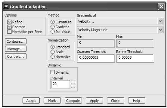
2. In the main FLUENT menu, choose Adapt>Gradient. In the new Gradient Adaption window, select Gradients of Velocity.
3. Select the Compute option. Minimum and maximum velocity gradients will appear in the window.
4. As a good rule of thumb, set the Refine Threshold to about 1/10 of the maximum gradient. Enter this values in the appropriate text box.
5. Click Mark. The main FLUENT window will display how many cells have been selected for refining and coarsening. The coarsening cells can be ignored since FLUENT is unable to coarsen the original grid – it can only refine the original grid.
6. Optional: If you want to see where the grid will be adapted, click Manage>Display. Areas destined for grid refinement will be highlighted. (You may need to zoom out to see this better.)
7. Back in the Gradient Adaption window, choose Adapt>Yes. The main FLUENT window will display some information about the grid adaptation.
8. The Gradient Adaption window can be closed at this point. Or, if you prefer – move it somewhere on the screen where it can be accessed again, since we will need it again later.
9. Optional: To see what the refined grid looks like, choose Display-Mesh from the main FLUENT menu, highlight interior-surface body, and Display. (You may need to zoom in close to the wall to see more clearly.) You should see some new cells near the wall (especially near the leading edge of the flat plate) where velocity gradients are highest.
10. Choose Solve>Run Calculation from the main FLUENT menu to reopen the Run Calculation sub-window. Change Number of Iterations to about 500, and then choose Calculate>OK.
11. After the iterations, check to see how the solution is progressing. In the main FLUENT menu, choose Display>Graphics and Animations>Vectors>Set Up>Display. The graphical display window will show the velocity vectors. They should be closer together in regions where the mesh was refined.
12. Under Surfaces, select only inlet, profile0.10, profile0.30, and outlet. Then choose Display.
13. Zoom in (use MMB lower left to upper right) or out (use MMB upper right to lower left) and move (using MMB where you want to center the view) as necessary to see all four velocity profiles.
14. Change the velocity vector scale to about 10 to see the profiles more clearly. Choose Display. The growth of the boundary layer should be apparent. Close the Vectors window.

Iterate towards a solution

1. At this point, the boundary layer should be reasonable, but more grid refinement and iteration may be required. As a general rule of thumb, if there are less than about 10 data points within the thickness of the boundary layer at the outlet profile location, the grid should be refined again.
2. Following the procedure outlined previously in the section called “Refine the mesh and iterate some more,” refine the grid and reiterate as necessary to obtain a final solution. Each time you adapt the grid, you must recalculate the gradients (Compute), readjust the refine threshold (again, it should be set to about 1/10 of the maximum gradient), Mark, Adapt>Yes.
3. Iterate at least 300 to 500 iterations after each grid adaption. The residuals will rise dramatically after an adaption, but will decay as the solution adjusts itself to the newly refined grid.
4. Caution: Don’t adapt too much, or the computations will take too much CPU time. Note that every time you refine the grid, the computer must calculate the flow field at more grid points, requiring longer for each successive iteration.
5. After refinement and iteration, look at the velocity profiles again, following the procedure discussed previously in the section called “Examine the velocity profiles in detail.”
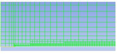
6. Adapt several times until there are at least 8 to 10 data points within the boundary layer at the outlet. A close-up view of a reasonable final mesh is shown to the right; notice the mesh refinement near the leading edge of the plate.
7. When finished adapting, run several hundred iterations until the residuals level off, or until the convergence criteria are reached.

Calculate the drag force and drag coefficient on the body

1. In order to calculate drag coefficient correctly, the proper reference values for area, velocity, and other settings need to be defined. In the main FLUENT menu, go to Report>Reference Values. A sub-window called Reference Values appears. The proper reference area to use is the planform area of the plate, defined as the area seen from above, in this case L times b, where L is the plate length (0.5 m) and b is the depth or span of the plate. In a 2D calculation, FLUENT assumes unit depth (b = 1.0 m) for convenience so that drag force is per unit depth. Depth should already be set to 1.0 m by default.
2. Change Area to “0.5” m2 (L times b), change Velocity to “0.1” m/s (the freestream velocity of the flow), and change Length to “0.5” m (L, the length of the flat plate).
3. Unfortunately, the reference values for density and viscosity are those of air, the default fluid, even though we defined our working fluid as liquid water. Change Density and Viscosity to their proper values. (These values for liquid water should have been written down previously, but can also be found from Define/Materials, and select water-liquid, and Create/Edit.)
4. In the main FLUENT menu, choose Report>Result Reports>Forces>Set Up. In the window that pops up, under Wall Zones, select only the plate. You will need to enter the components of the force vector. These are the x and y components of a unit vector pointing in the direction of the desired force. Here, set the x-component to 1 and the y-component to 0, causing FLUENT to calculate the force (the drag force) acting on the wall in the x-direction, defined as parallel to the freestream direction.
5. Print to perform the calculation. The results will be printed to the main FLUENT window.
6. Write down the total drag force and drag coefficient on the flat plate.
7. To exit the Force Reports window, click Close.

Save your calculations and exit FLUENT

1. In the main FLUENT menu, select File>Save Project. Then, File>Export>Case & Data. Click OK. It is okay to overwrite the files, so click OK again.
2. Exit FLUENT by File>Close FLUENT. Make sure the option to store the results is turned on. Click OK. This will return you to Workbench.
3. In Workbench, choose Update Project. After some calculations, check marks should appear on all components of the Fluid Flow (FLUENT) template in Project Schematic.

Previous answers to this question

---

Get The Answer